6. How to Solve ODEs with Rate Law Functions

In general, ReactionRule describes a mass action kinetics with no more than two reactants. In case of a reaction with a complecated rate law, ReactionRule could be extensible with ReactionRuleDescriptor. Here, we explan the use of ReactionRuleDescriptor especially for ode.

%matplotlib inline
from ecell4 import *
from ecell4_base import *
from ecell4_base.core import *

6.1. ReactionRuleDescriptor

ReactionRule defines reactants, products, and a kinetic rate.

rr1 = ReactionRule()
rr1.add_reactant(Species("A"))
rr1.add_reactant(Species("B"))
rr1.add_product(Species("C"))
rr1.set_k(1.0)
print(len(rr1.reactants()))  # => 2
print(len(rr1.products()))  # => 1
print(rr1.k())  # => 1.0
print(rr1.as_string())  # => A+B>C|1
print(rr1.has_descriptor())  # => False

2
1
1.0
A+B>C|1
False

In addition to that, ReactionRule could be extensible with ReactionRuleDescriptor.

desc1 = ReactionRuleDescriptorMassAction(1.0)
print(desc1.k())
rr1.set_descriptor(desc1)

1.0

ReactionRuleDescriptor is accessible from ReactionRule.

print(rr1.has_descriptor())
print(rr1.get_descriptor())
print(rr1.get_descriptor().k())

True
<ecell4_base.core.ReactionRuleDescriptorMassAction object at 0x154e09b03190>
1.0

ReactionRuleDescriptor can store stoichiometric coefficients for each reactants:

desc1.set_reactant_coefficient(0, 2)  # Set a coefficient of the first reactant
desc1.set_reactant_coefficient(1, 3)  # Set a coefficient of the second reactant
desc1.set_product_coefficient(0, 4)  # Set a coefficient of the first product
print(rr1.as_string())

2*A+3*B>4*C|1

You can get the list of coefficients in the following way:

print(desc1.reactant_coefficients())  # => [2.0, 3.0]
print(desc1.product_coefficients())  # => [4.0]

[2.0, 3.0]
[4.0]

Please be careful that ReactionRuleDescriptor works properly only with ode.

6.2. ReactionRuleDescriptorPyFunc

ReactionRuleDescriptor provides a function to calculate a derivative (flux or velocity) based on the given values of Species. In this section, we will explain the way to define your own kinetic law.

rr1 = ReactionRule()
rr1.add_reactant(Species("A"))
rr1.add_reactant(Species("B"))
rr1.add_product(Species("C"))
print(rr1.as_string())

A+B>C|0

First, define a rate law function as a Python function. The function must accept six arguments and return a floating number. The first and second lists contain a value for each reactants and products respectively. The third and fourth represent volume and time. The coefficients of reactants and products are given in the last two arguments.

def ratelaw(r, p, v, t, rc, pc):
    return 1.0 * r[0] * r[1] - 2.0 * p[0]

ReactionRuleDescriptorPyFunc accepts the function.

desc1 = ReactionRuleDescriptorPyfunc(ratelaw, 'test')
desc1.set_reactant_coefficients([1, 1])
desc1.set_product_coefficients([1])
rr1.set_descriptor(desc1)
print(desc1.as_string())
print(rr1.as_string())

test
1*A+1*B>1*C|0

A lambda function is available too.

desc2 = ReactionRuleDescriptorPyfunc(lambda r, p, v, t, rc, pc:  1.0 * r[0] * r[1] - 2.0 * p[0], 'test')
desc2.set_reactant_coefficients([1, 1])
desc2.set_product_coefficients([1])
rr1.set_descriptor(desc2)
print(desc1.as_string())
print(rr1.as_string())

test
1*A+1*B>1*C|0

To test if the function works properly, evaluate the value with ode.World.

w = ode.World()
w.set_value(Species("A"), 10)
w.set_value(Species("B"), 20)
w.set_value(Species("C"), 30)

print(w.evaluate(rr1))  # => 140 = 1 * 10 * 20 - 2 * 30

140.0

6.3. NetworkModel

NetworkModel accepts ReactionRules with and without ReactionRuleDescriptor.

m1 = NetworkModel()
rr1 = create_unbinding_reaction_rule(Species("C"), Species("A"), Species("B"), 3.0)
m1.add_reaction_rule(rr1)
rr2 = create_binding_reaction_rule(Species("A"), Species("B"), Species("C"), 0.0)
desc1 = ReactionRuleDescriptorPyfunc(lambda r, p, v, t, rc, pc: 0.1 * r[0] * r[1], "test")
desc1.set_reactant_coefficients([1, 1])
desc1.set_product_coefficients([1])
rr2.set_descriptor(desc1)
m1.add_reaction_rule(rr2)

You can access to the list of ReactionRules in NetworkModel via its member reaction_rules().

print([rr.as_string() for rr in m1.reaction_rules()])

['C>A+B|3', '1*A+1*B>1*C|0']

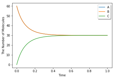
Finally, you can run simulations in the same way with other solvers as follows:

run_simulation(1.0, model=m1, y0={'A': 60, 'B': 60})

Modeling with Python decorators is also available by specifying a function instead of a rate (floating number). When a floating number is set, it is assumed to be a kinetic rate of a mass action reaction, but not a constant velocity.

from functools import reduce
from operator import mul

with reaction_rules():
    A + B == C | (lambda r, *args: 0.1 * reduce(mul, r), 3.0)

m1 = get_model()

For the simplicity, you can directory defining the equation with Species names as follows:

with reaction_rules():
    A + B == C | (0.1 * A * B, 3.0)

m1 = get_model()

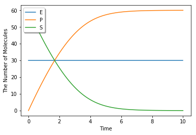
When you call a Species (in the rate law) which is not listed as a reactant or product, it is automatically added to the list as an enzyme.

with reaction_rules():
    S > P | 1.0 * E * S / (30.0 + S)

m1 = get_model()
print(m1.reaction_rules()[0].as_string())
print(m1.reaction_rules()[0].get_descriptor().as_string())

1*S+1*E>1*P+1*E|0
((1.0*E*S)/(30.0+S))

where E in the equation is appended to both reacant and product lists.

run_simulation(10.0, model=m1, y0={'S': 60, 'E': 30})

Please be careful about typo in Species’ name. When you make a typo, it is unintentionally recognized as a new enzyme:

with reaction_rules():
    A13P2G > A23P2G | 1500 * A13B2G  # typo: A13P2G -> A13B2G

m1 = get_model()
print(m1.reaction_rules()[0].as_string())

1*A13P2G+1*A13B2G>1*A23P2G+1*A13B2G|0

When you want to disable the automatic declaration of enzymes, inactivate util.decorator.ENABLE_IMPLICIT_DECLARATION. If its value is False, the above case will raise an error:

util.decorator.ENABLE_IMPLICIT_DECLARATION = False

try:
    with reaction_rules():
        A13P2G > A23P2G | 1500 * A13B2G
except RuntimeError as e:
    print(repr(e))

util.decorator.ENABLE_IMPLICIT_DECLARATION = True

RuntimeError('[A13B2G] is unknown [(1500*{0})].',)

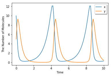
Although E-Cell4 is specialized for a simulation of biochemical reaction network, by using a synthetic reaction rule, ordinary differential equations can be translated intuitively. For example, the Lotka-Volterra equations:

\[\begin{split}\frac{dx}{dt} = Ax - Bxy\\\frac{dy}{dt} = -Cx + Dxy\end{split}\]

where \(A=1.5, B=1, C=3, D=1, x(0)=10, y(0)=5\), are solved as follows:

with reaction_rules():
    A, B, C, D = 1.5, 1, 3, 1

    ~x > x | A * x - B * x * y
    ~y > y | -C * y + D * x * y

run_simulation(10, model=get_model(), y0={'x': 10, 'y': 5})

6.4. References in a Rate Law

Here, we exlain the details in the rate law definition.

First, when you use simpler definitions of a rate law with Species, only a limited number of mathematical functions (e.g. exp, log, sin, cos, tan, asin, acos, atan, and pi) are available there even if you declare the function outside the block.

try:
    from math import erf

    with reaction_rules():
        S > P | erf(S / 30.0)
except TypeError as e:
    print(repr(e))

TypeError('must be real number, not DivExp',)

This error happens because erf is tried to be evaluated agaist S / 30.0, which is not a floating number. In contrast, the following case is acceptable:

from math import erf

with reaction_rules():
    S > P | erf(2.0) * S

m1 = get_model()
print(m1.reaction_rules()[0].get_descriptor().as_string())

(0.9953222650189527*S)

where only the result of erf(2.0), 0.995322265019, is passed to the rate law. Thus, the rate law above has no reference to the erf function. Similarly, a value of variables declared outside is acceptable, but not as a reference.

kcat, Km = 1.0, 30.0

with reaction_rules():
    S > P | kcat * E * S / (Km + S)

m1 = get_model()
print(m1.reaction_rules()[0].get_descriptor().as_string())
kcat = 2.0  # This doesn't affect the model
print(m1.reaction_rules()[0].get_descriptor().as_string())

((1.0*E*S)/(30.0+S))
((1.0*E*S)/(30.0+S))

Even if you change the value of a variable, it does not affect the rate law.

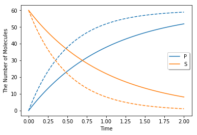
On the other hand, when you use your own function to define a rate law, it can hold a reference to variables outside.

k1 = 1.0

with reaction_rules():
    S > P | (lambda r, *args: k1 * r[0])  # referring k1

m1 = get_model()

obs1 = run_simulation(2, model=m1, y0={"S": 60}, return_type='observer')
k1 = 2.0  # This could change the result
obs2 = run_simulation(2, model=m1, y0={"S": 60}, return_type='observer')

viz.plot_number_observer(obs1, '-', obs2, '--')

However, in this case, it is better to make a new model for each set of parameters.

def create_model(k):
    with reaction_rules():
        S > P | k

    return get_model()

obs1 = run_simulation(2, model=create_model(k=1.0), y0={"S": 60}, return_type='observer')
obs2 = run_simulation(2, model=create_model(k=2.0), y0={"S": 60}, return_type='observer')
viz.plot_number_observer(obs1, '-', obs2, '--')

6.5. More about ode

In ode.World, a value for each Species is a floating number. However, for the compatibility, the common member num_molecules and add_molecules regard the value as an integer.

w = ode.World()
w.add_molecules(Species("A"), 2.5)
print(w.num_molecules(Species("A")))

2

To set/get a real number, use set_value and get_value:

w.set_value(Species("B"), 2.5)
print(w.get_value(Species("A")))
print(w.get_value(Species("B")))

2.0
2.5

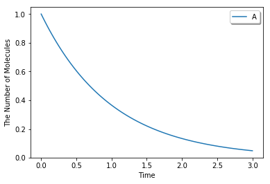
As a default, ode.Simulator employs the Rosenblock method, called ROSENBROCK4_CONTROLLER, to solve ODEs. In addition to that, two solvers, EULER and RUNGE_KUTTA_CASH_KARP54, are available. ROSENBROCK4_CONTROLLER and RUNGE_KUTTA_CASH_KARP54 adaptively change the step size during time evolution due to error controll, but EULER does not.

with reaction_rules():
    A > ~A | 1.0

m1 = get_model()

w1 = ode.World()
w1.set_value(Species("A"), 1.0)
sim1 = ode.Simulator(w1, m1, ode.EULER)
sim1.set_dt(0.01) # This is only effective for EULER
sim1.run(3.0, obs1)

ode.Factory also accepts a solver type and a default step interval.

run_simulation(3.0, model=m1, y0={"A": 1.0}, solver=('ode', ode.EULER, 0.01))

See also examples listed below:

• Glycolysis of Human Erythrocytes
• Drosophila Circadian Clock
• Attractors