1. Brief Tour of E-Cell4 Simulations

First of all, you have to load the E-Cell4 library:

%matplotlib inline
from ecell4 import *
from ecell4_base.core import *

1.1. Quick Demo

There are three fundamental components consisting of E-Cell System version 4, which are Model, World, and Simulator. These components describe concepts in simulation.

• Model describes a problem to simulate as its name suggests.
• World describes a state, e.g. an initial state and a state at a time-point.
• Simulator describes a solver.

Model is independent from solvers. Every solver can share a single Model instance. Each solver alogrithm has a corresponding pair of World and Simulator (these pairs are capsulized into Factory class). World is not necessarily needed to be bound to Model and Simulator, but Simulator needs both Model and World.

Before running a simulation, you have to make a Model. E-Cell4 supports multiple ways to buld a Model (See 2. How to Build a Model local ipynb readthedocs). Here, we explain the simplest way using the with statement with reaction_rules:

with reaction_rules():
    A + B > C | 0.01  # equivalent to create_binding_reaction_rule
    C > A + B | 0.3   # equivalent to create_unbinding_reaction_rule

m1 = get_model()
print(m1)

<ecell4_base.core.NetworkModel object at 0x14fdde89bb90>

Please remember to write parentheses () after reaction_rules. Here, a Model with two ReactionRules named m1 was built. Lines in the with block describe ReactionRules, a binding and unbinding reaction respectively. A kinetic rate for the mass action reaction is defined after a separator |, i.e. 0.01 or 0.3. In the form of ordinary differential equations, this model can be described as:

\[[\mathrm{A}]'=[\mathrm{B}]'=-[\mathrm{C}]=-0.01[\mathrm{A}][\mathrm{B}]+0.3[\mathrm{C}]\]

For more compact description, A + B == C | (0.01, 0.3) is also acceptable.

E-Cell4 has a simple interface for running simulation on a given model, called run_simulation. This enables for you to run simulations without instanciate World and Simulator by yourself. To solve this model, you have to give a volume, an initial value for each Species and duration of time:

run_simulation(10.0, model=m1, y0={'A': 60, 'B': 60}, volume=1.0)

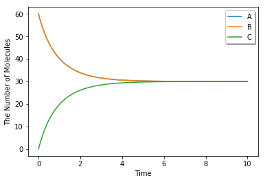
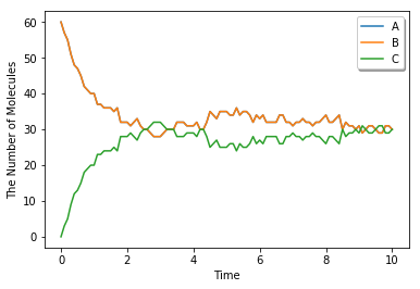
To switch simulation algorithm, you only need to give the type of solver (ode is used as a default) as follows:

run_simulation(10.0, model=m1, y0={'A': 60, 'B': 60}, solver='gillespie')

1.2. Spatial Simulation and Visualization

E-Cell4 now supports multiple spatial simulation algorithms, egfrd, spatiocyte and meso. In addition to the model used in non-spatial solvers (ode and gillespie), these spatial solvers need extra information about each Species, i.e. a diffusion coefficient and radius.

The with statement with species_attributes is available to describe these properties:

with species_attributes():
    A | B | C | {'radius': 0.005, 'D': 1}  # 'D' is for the diffusion coefficient

with reaction_rules():
    A + B == C | (0.01, 0.3)

m2 = get_model()

Species attributes could be a string, boolean, integer or floating number.

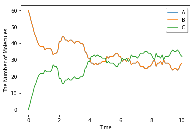
Now you can run a spatial simulation in the same way as above (in the case of egfrd, the time it takes to finish the simulation will be longer):

run_simulation(10.0, model=m2, y0={'A': 60, 'B': 60}, solver='meso')

Structure (e.g. membrane, cytoplasm and nucleus) is only supported by spatiocyte and meso for now. For the simulation, location and dimension that each species belongs to must be specified in its attribute.

with species_attributes():
    A | {'D': 1, 'location': 'S', 'dimension': 3}  # 'S' is a name of the structure
    S | {'dimension': 3}

m3 = get_model()  # with no reactions

E-Cell4 supports primitive shapes as a structure like Sphere:

sphere = Sphere(Real3(0.5, 0.5, 0.5), 0.48)  # a center position and radius

E-Cell4 provides various kinds of Observers which log the state during a simulation. In the following two observers are declared to record the position of the molecule. FixedIntervalTrajectoryObserver logs a trajectory of a molecule, and FixedIntervalHDF5Observer saves World to a HDF5 file at the given time interval:

obs1 = FixedIntervalTrajectoryObserver(1e-3)
obs2 = FixedIntervalHDF5Observer(0.1, 'test%02d.h5')

run_simulation can accept structures and observers as arguments structure and observers (see also help(run_simulation)):

run_simulation(1.0, model=m3, y0={'A': 60}, structures={'S': sphere},
               solver='spatiocyte', observers=(obs1, obs2), return_type=None)

E-Cell4 has a function to visualize the world which is also capable of interactive visualization named viz.plot_world. viz.plot_world plots positions of molecules in 3D. In addition, by using load_world, you can easily restore the state of World from a HDF5 file:

# viz.plot_world(load_world('test00.h5'), species_list=['A'])
viz.plot_world(load_world('test00.h5'), species_list=['A'], interactive=True)

Also, for FixedIntervalTrajectoryObserver,viz.plot_trajectory generates a plot of the trajectory. (Again, it is possible to generate interactive plots.):

# viz.plot_trajectory(obs1)
viz.plot_trajectory(obs1, interactive=True)

For more details, see 5. How to Log and Visualize Simulations local ipynb readthedocs.